Commercial LOS
SQL
- Calculate length of stay (LOS) from admission and discharge dates.
- Filter to CLD hospitals, MS-DRG codes, commercial plans, inpatient claims, and patients under 65.
- Use TQ IPPS grouper to assign MS-DRG codes (
ipps_grouper_drgs)
- Aggregate commercial LOS by provider, state, and national levels.
- Use geometric mean (GLOS) and median LOS metrics.
- Join with CMS ALOS and GLOS for comparison.
Query 1
CREATE TABLE tq_intermediate.cld_utils.komodo_inpatient_encounters_los AS
WITH

------------------
-- CLD INPUTS
------------------
provider_spine AS (
    SELECT
        DISTINCT
        provider_id,
        npi_value AS npi
    FROM
        tq_dev.internal_dev_csong_cld_v2_0_0.prod_rollup_provider,
        UNNEST(npi) AS t(npi_value)
    WHERE
        provider_id IS NOT NULL
        AND provider_type LIKE '%Hospital%'
),
code_spine AS (
    SELECT
        billing_code AS diagnosis_group
    FROM
        tq_dev.internal_dev_csong_cld_v2_0_0.prod_rollup_code
    WHERE
        billing_code_type = 'MS-DRG'
),

------------------
-- Komodo Data:
-- filter to CLD providers and codes
-- include only commercial plans
-- inpatient claims only
-- age < 65
------------------
komodo_headers AS (
    SELECT
        mh.encounter_key,
        mh.patient_dob,
        ps.provider_id,
        mh.admission_date,
        mh.discharge_date,
        DATE_DIFF('day', mh.admission_date, mh.discharge_date) AS los,
        COALESCE(ig.new_drg, SUBSTR(mh.diagnosis_group, 2)) as drg
    FROM tq_intermediate.external_komodo.medical_headers mh
    JOIN tq_intermediate.external_komodo.ipps_grouper_drgs ig
        ON mh.encounter_key = ig.encounter_key
    JOIN code_spine
        ON COALESCE(ig.new_drg, SUBSTR(mh.diagnosis_group, 2)) = code_spine.diagnosis_group
    JOIN provider_spine ps
        ON mh.hco_1_npi = ps.npi
    JOIN tq_intermediate.external_komodo.plans kp
        ON mh.kh_plan_id = kp.kh_plan_id
        AND kp.insurance_group = 'COMMERCIAL'
    WHERE
        claim_type_code = 'I'
        AND YEAR(patient_dob) > 1960
)
SELECT
    h.encounter_key,
    h.provider_id,
    h.drg as billing_code,
    'MS-DRG' as billing_code_type,
    admission_date,
    discharge_date,
    los,
    h.patient_dob
FROM komodo_headers h
WHERE los > 0
Query 2
CREATE TABLE tq_intermediate.cld_utils.komodo_inpatient_los AS
WITH

-- Provider-level LOS stats
df AS (
    SELECT
        los.provider_id,
        sp.provider_name,
        sp.provider_state,
        billing_code,
        count(*) AS n_encounters,
        EXP(AVG(LN(los))) AS glos,
        APPROX_PERCENTILE(los, 0.5) AS median_los,
        AVG(los) AS avg_los,
        ANY_VALUE(cms.glos) AS cms_glos,
        ANY_VALUE(cms.alos) AS cms_alos
    FROM tq_intermediate.cld_utils.komodo_inpatient_encounters_los los
    LEFT JOIN tq_production.spines.spines_provider sp
        ON los.provider_id = sp.provider_id
    LEFT JOIN tq_production.reference_legacy.ref_cms_msdrg cms
        ON billing_code = cms.msdrg
    WHERE
        los < 50
    GROUP BY 1,2,3,4
),

-- National LOS stats
commercial_median AS (
    SELECT
        billing_code,
        EXP(AVG(LN(los))) AS glos,
        APPROX_PERCENTILE(los, 0.5) AS median_los
    FROM tq_intermediate.cld_utils.komodo_inpatient_encounters_los
    GROUP BY 1
),

-- State-specific LOS stats
provider_state AS (
    SELECT
        provider_state,
        billing_code,
        EXP(AVG(LN(los)))AS glos,
        APPROX_PERCENTILE(los, 0.5) AS median_los
    FROM tq_intermediate.cld_utils.komodo_inpatient_encounters_los los
    LEFT JOIN tq_production.spines.spines_provider sp
        ON los.provider_id = sp.provider_id
    GROUP BY 1,2
)

-- Final selection
SELECT
    df.*,
    cm.glos AS commercial_national_glos,
    cm.median_los AS commercial_national_median_los,
    ps.glos AS provider_state_median_glos,
    ps.median_los AS provider_state_median_los
FROM df
LEFT JOIN commercial_median cm
    ON df.billing_code = cm.billing_code
LEFT JOIN provider_state ps
    ON df.billing_code = ps.billing_code
    AND df.provider_state = ps.provider_state
Analysis
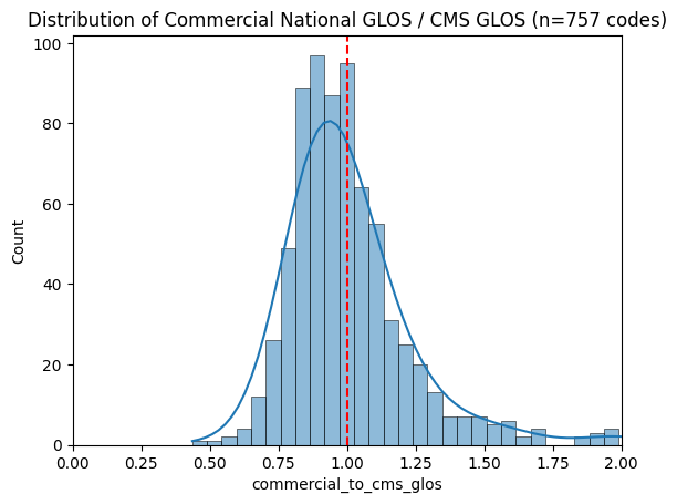
- Nationally, the geometric length of stay (GLOS) for commercial inpatient encounters is slightly lower than the national average. But the difference is small.
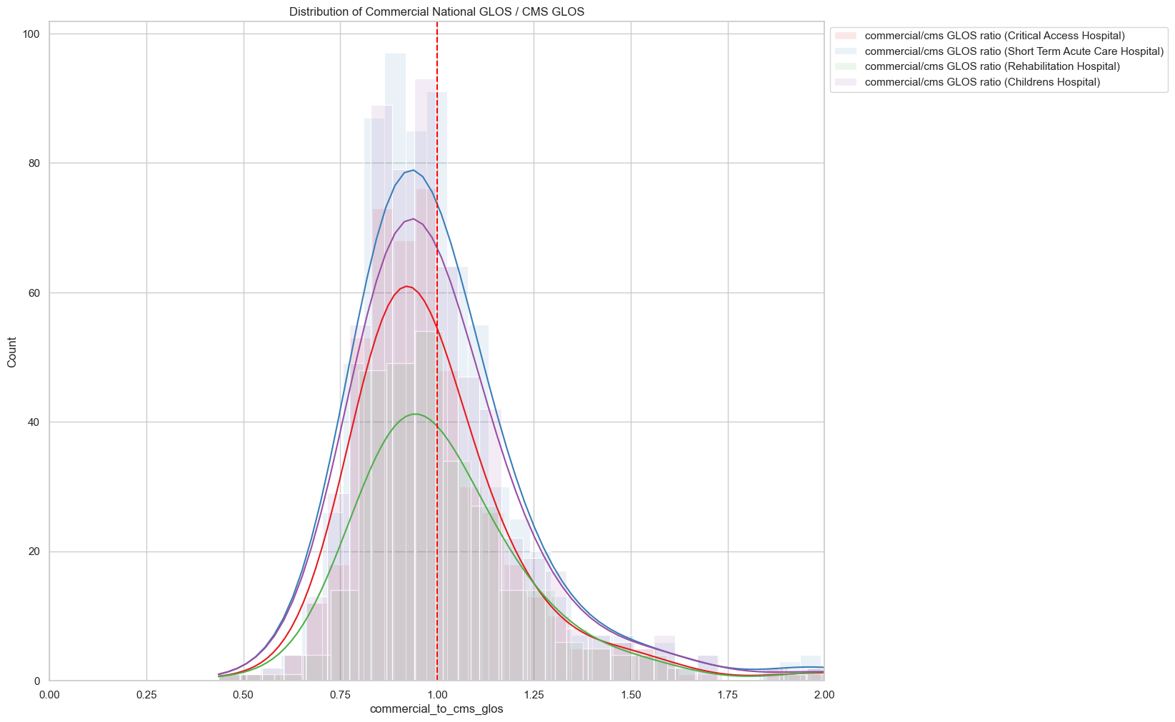
By provider type:
- Codes where commercial GLOS and CMS GLOS are most different:
Commercial GLOS > CMS GLOS:
Commercial GLOS < CMS GLOS:
Code for Plots:
# %% [markdown]
"""
Evaluate
"""
# %%
df = pd.read_sql(f"""
SELECT *
FROM tq_intermediate.cld_utils.komodo_inpatient_los
""", con=trino_conn)
# %%
# distribution of n_encounters
ax = sns.histplot(df['n_encounters'][df['n_encounters']<110].sample(1000))
ax.set_xlim(0, 100)
# %%
# distribution of commercial national GLOS / cms GLOS
dftmp = df.drop_duplicates(subset='billing_code')
dftmp['commercial_to_cms_glos'] = dftmp['commercial_national_glos'] / dftmp['cms_glos']
ax = sns.histplot(
dftmp['commercial_to_cms_glos'],
kde=True,
label='commercial/cms GLOS ratio'
)
ax.set_xlim(0, 2)
plt.title('Distribution of Commercial National GLOS / CMS GLOS (n=757 codes)')
plt.axvline(1, color='red', linestyle='--')
# %%
# distribution by provider type
sns.set_theme(style='whitegrid', rc={'figure.figsize': (14, 12)})
colormap = sns.color_palette("Set1", n_colors=len(df['provider_type'].unique()))
for provider_type in df['provider_type'].unique():
dftmp = df[df['provider_type'] == provider_type].drop_duplicates(subset='billing_code')
dftmp['commercial_to_cms_glos'] = dftmp['commercial_national_glos'] / dftmp['cms_glos']
ax = sns.histplot(
dftmp['commercial_to_cms_glos'],
kde=True,
label=f'commercial/cms GLOS ratio ({provider_type})',
color=colormap[df['provider_type'].unique().tolist().index(provider_type)],
# don't fill bars
fill=0.1,
alpha=0.1,
)
ax.set_xlim(0, 2)
plt.title('Distribution of Commercial National GLOS / CMS GLOS')
plt.axvline(1, color='red', linestyle='--')
plt.legend(loc='upper left', bbox_to_anchor=(1, 1))
# %%
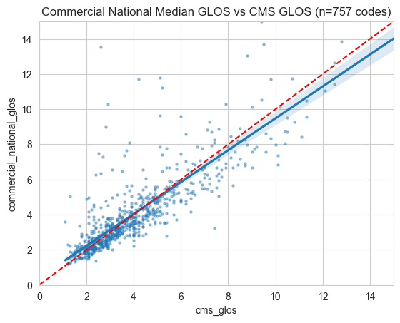
# commercial national glos vs cms glos
ax = sns.regplot(
data=df.drop_duplicates(subset='billing_code'),
x='cms_glos',
y='commercial_national_glos',
scatter_kws={'alpha': 0.4, 's': 5},
)
plt.plot([0, 15], [0, 15], color='red', linestyle='--', label='y=x')
plt.title('Commercial National Median GLOS vs CMS GLOS (n=757 codes)')
ax.set_ylim(0,15)
ax.set_xlim(0,15)
# %%
# individual providers
ax = sns.regplot(
data=df.loc[df['n_encounters']>100],
x='cms_glos',
y='glos',
scatter_kws={'alpha': 0.1, 's': 5},
)
ax.set_ylim(0,15)
ax.set_xlim(0,15)
plt.title('Provider-Specific GLOS vs CMS GLOS for Codes with >100 Encounters')
plt.plot([0, 15], [0, 15], color='red', linestyle='--', label='y=x')
plt.legend()
# %%
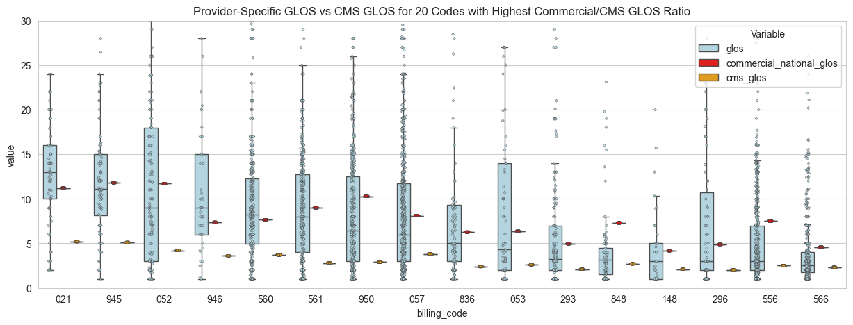
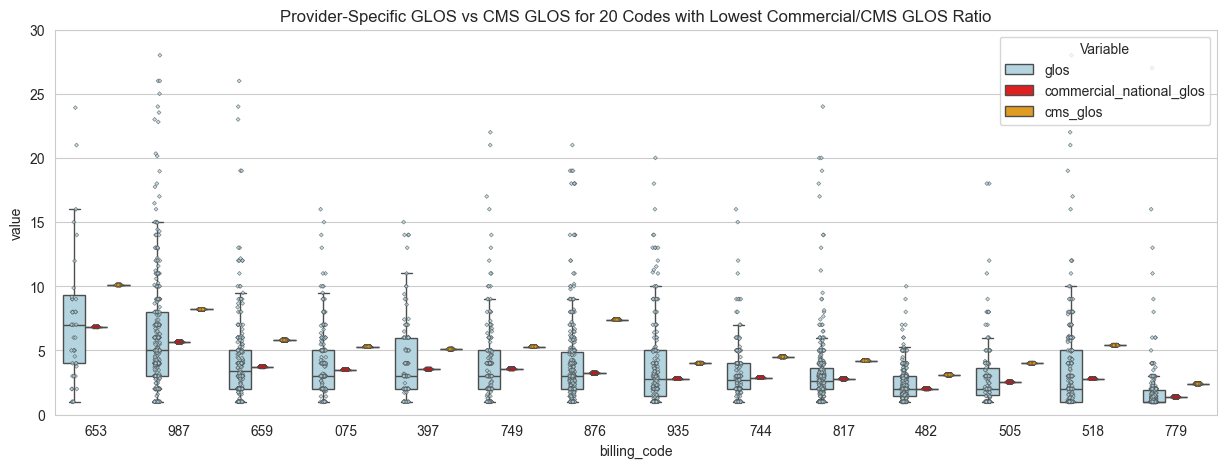
# compare codes with high commercial national GLOS / CMS GLOS ratio
code_sums = df.groupby('billing_code').agg({'n_encounters': 'sum'})
dfboxplot = (
df
.loc[df['billing_code'].isin((code_sums.loc[code_sums['n_encounters']>100].index))]
.loc[
df['billing_code'].isin(dftmp.sort_values('commercial_to_cms_glos', ascending=True).head(20)['billing_code'])
]
)
dfboxplot = (
dfboxplot
.melt(id_vars=['provider_id', 'billing_code'], value_vars=['glos', 'commercial_national_glos', 'cms_glos'])
)
order = (
dfboxplot
.loc[dfboxplot['variable'] == 'glos']
.groupby(['billing_code', 'variable'])
.value.median()
.reset_index()
.sort_values(['variable', 'value'], ascending=[True, False])
['billing_code']
)
sns.set_style('whitegrid')
plt.figure(figsize=(15, 5))
ax = sns.boxplot(
data=dfboxplot,
order=order.unique(),
x='billing_code',
y='value',
hue='variable',
showfliers=False,
palette=['lightblue', 'red', 'orange'],
)
sns.stripplot(
data=dfboxplot,
order=order.unique(),
x='billing_code',
y='value',
hue='variable',
dodge=True,
alpha=0.7,
palette=['lightblue', 'red', 'orange'],
marker='D',
edgecolor='gray',
linewidth=0.5,
size=2
)
ax.set_ylim(0, 30)
# Remove duplicate legend
handles, labels = plt.gca().get_legend_handles_labels()
plt.legend(handles[:3], labels[:3], title="Variable", loc='upper right')
plt.title('Provider-Specific GLOS vs CMS GLOS for 20 Codes with Lowest Commercial/CMS GLOS Ratio')
Takeaways
- On average, commercial GLOS and CMS glos are similar. The differences in GLOS and CMS GLOS would not meaningfully impact aggregate provider comparisons.
- Commercial GLOS can be 50% to 150% of CMS GLOS. Most codes are within 20% of CMS GLOS.
- Variability at the provider-level is higher. But there are lower sample sizes for many providers. It's unclear if the variability is due to noise or true differences in care patterns.